

Better Steering with Less Data: Kinematic Priors Guide Trajectory Prediction
Table of Links
Abstract and I. Introduction
II. Related Work
III. Kinematics of Traffic Agents
IV. Methodology
V. Results
VI. Discussion and Conclusion, and References
VII. Appendix
V. RESULTS
In this section, we show experiments that highlight the effect of kinematic priors on performance. We implement kinematic priors on state-of-the-art method Motion Transformer (MTR) [7], which serves as our baseline method.
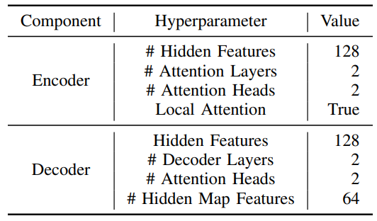
\ Hardware. We train all experiments on eight RTX A5000 GPUs, with 64 GB of memory and 32 CPU cores. Experiments on the full dataset are trained for 30 epochs, while experiments with the smaller dataset are trained for 50 epochs. Additionally, we downscale the model from its original size of 65 million parameters to 2 million parameters and re-train all models under these settings for fair comparison. Furthermore, we re-implement Deep Kinematic Models (DKM) [1] to contextualize our probabilistic method against deterministic methods, as the official implementation is not publicly available. DKM is implemented against the same backbone as vanilla MTR and our models. More details on training hyperparameters can be found in Table VIII of the appendix, which can also be found on the project website.
\
A. Performance on Waymo Motion Prediction Dataset
We evaluate the baseline model and all kinematic formulations on the Waymo Motion Prediction Dataset [8]. The Waymo dataset consists of over 100,000 segments of traffic, where each scenario contains multiple agents of three classes: vehicles, pedestrians, and cyclists. The data is collected from high-quality, high-resolution sensors that sample traffic states at 10 Hz. The objective is, given 1 second of trajectory history for each vehicle, to predict trajectories for the next 8 seconds. For simplicity, we use the bicycle kinematic model for all three classes and leave discerning between the three, especially for pedestrians, for future work.
\ We evaluate our model’s performance on Mean Average Precision (mAP), Minimum Average Displacement Error (minADE), minimum final displacement error (minFDE), and Miss Rate, similarly to [8]. We reiterate their definitions below for convenience.
\ • Mean Average Precision (mAP): mAP is computed across all classes of trajectories. The classes include straight, straight-left, straight-right, left, right, left uturn, right u-turn, and stationary. For each prediction, one true positive is chosen based on the highest confidence trajectory within a defined threshold of the ground truth trajectory, while all other predictions are assigned a false positive. Intuitively, the mAP metric describes prediction precision while accounting for all trajectory class types. This is beneficial especially when there is an imbalance of classes in the dataset (e.g., there may be many more straight-line trajectories in the dataset than there are right u-turns).
\ ![TABLE II: Performance comparison on vehicles for each kinematic formulation versus SOTA in a small dataset setting. We train models on 1% of the original Waymo Motion Dataset and use the same full evaluation set as that in Table I. We see pronounced improvements in performance metrics in settings with significantly less data available, with a nearly 13% mAP performance gain over the baseline and nearly 50% mAP performance gain compared to deterministic kinematic method from DKM [1] across most formulations.](https://cdn.hackernoon.com/images/fWZa4tUiBGemnqQfBGgCPf9594N2-44033ad.png)
\ 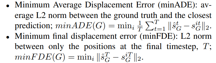
\ • Miss Rate: The number of predictions lying outside a reasonable threshold from the ground truth. The miss rate first describes the ratio of object predictions lying outside a threshold from the ground truth to the total number of agents predicted.
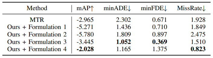
\ We show results for the Waymo Motion dataset in Table I, where we compared performance across two baselines, MTR [7] and DKM [1], and all formulations. From these results, we observe the greatest improvement over the baseline with Formulation 3, which involves the first-order velocity and heading components. We observe that the benefit of our method in full-scale training settings diminishes. This performance gap closing may be due to the computational complexity of the network, the large dataset, and or the long supervised training time out-scaling benefits provided by applying kinematic constraints. However, deploying models in the wild may not necessarily have such optimal settings, especially in cases of sparse data or domain transfer. Thus, we also consider the effects of suboptimal settings for trajectory prediction, as we hypothesize that learning first or second-order terms provides information when data cannot. This is also motivated by problems in the real world, where sensors may not be as high-quality or specific traffic scenarios may not be so abundantly represented in data.
\
B. Performance on a Smaller Dataset Setting
We examine the effects of kinematic priors on a smaller dataset size. This is motivated by the fact driving datasets naturally have an imbalance of scenarios, where many samples are representative of longitudinal straight-line driving or stationary movement, and much less are representative of extreme lateral movements such as U-turns. Thus, large and robust benchmarks like the Waymo, Nuscenes, and Argoverse datasets are necessary for learning good models. However, large datasets are not always accessible depending on the setting. For example, traffic laws, road design, and natural dynamics vary by region. It would be infeasible to expect the same scale and robustness of data from every scenario in the world, and thus trajectory forecasting will run into settings with less data available.
\ We train the baseline model and all formulations on only 1% of the original Waymo dataset and benchmark their performance on 100% of the evaluation set in Table II. All experiments were trained over 50 epochs. In the small dataset setting, we observe that providing a kinematic prior in any form improves performance for minimum final displacement error (minFDE). Additionally, we observe better performance across all metrics for formulations 1, 2, and 1 with interpolation. Figure 4 shows how all kinematic formulations improve convergence speed over the baseline, with Formulation 4 (acceleration and steering) converging most quickly. Overall, Formulation 1 provides the greatest boost in mAP performance, with over 13% gain over the vanilla baseline and 50% over the deterministic baseline DKM, while Formulations 3 and 4 provide the greatest boost in distance metrics. In general, all formulations provide similar benefits in the small dataset setting, with the most general performance benefit coming from Formulation 3. While Formulation 4 also provides a comparable performance boost, the difference from Formulation 3 may be attributed to compounding error from second-order approximation. Interestingly, we note that modeling mean trajectories with kinematic priors is not enough to produce performance gain, as shown by the lower performance of DKM compared to vanilla MTR.
\ Compared to the results from Table I, the effects of kinematic priors in learning are more pronounced. Since kinematic priors analytically relate the position at one timestep to the position at the next, improvements in metrics may suggest that baseline models utilize a large amount of expressivity to model underlying kinematics. In backpropagation, optimization of one position further into the time horizon directly influences predicted positions at earlier timesteps via the kinematic model. Without the kinematic prior, the relation between timesteps may be implicitly related through neural network parameters. When the model lacks data to form a good model of how an agent moves through space, the kinematic model can help to compensate by modeling simple constraints.
\ 
\
C. Performance in the Presence of Noise
We also show how kinematic priors can influence performance in the presence of noise. This is inspired by the scenario where sensors may have a small degree of noise associated with measurements dependent on various factors, such as weather, quality, interference, etc.
\ We evaluate the models from Table III when input trajectories are perturbed by standard normal noise nϵ ∼ N (0, 1); results for performance degradation are shown in Table III.
\ We compute results in Table III by measuring the % of degradation of the perturbed evaluation from the corresponding original clean evaluation. We find that Formulation 4 from Section IV-B.4 with steering and acceleration components preserves the most performance in the presence of noise. This may be due to that second-order terms like acceleration are less influenced by perturbations on position, in addition to providing explicit bicycle-like constraints on vehicle movement. Additionally, distributions of acceleration are typically centered around zero regardless of how positions are distributed [33], which may provide more stability for learning.
\
VI. DISCUSSION AND CONCLUSION
In this paper, we present a simple method for including kinematic relationships in probabilistic trajectory forecasting. Kinematic priors can also be implemented for deterministic methods where linear approximations are not necessary. With nearly no additional overhead, we not only show improvement in models trained on robust datasets but also in suboptimal settings with small datasets and noisy trajectories, with up to 12% improvement in smaller datasets and 1% less performance degradation in the presence of noise for the full Waymo dataset. For overall performance improvement, we find Formulation 1 with velocity components to be the most beneficial and well-rounded to prediction performance.
\ When there is large-scale data to learn a good model of how vehicles move, we observe that the effects of kinematic priors are less pronounced. This is demonstrated by the less obvious improvements over the baseline in Table I compared to Table II; model complexity and dataset size will eventually out-scale the effects of the kinematic prior. With enough resources and high-quality data, trajectory forecasting models will learn to “reinvent the steering wheel”, or implicitly learn how vehicles move via the complexity of the neural network.
\ One limitation is that we primarily explore analysis in one-shot prediction; future work focusing on kinematic priors for autoregressive approaches would be interesting in comparison to one-shot models with kinematic priors, especially since autoregressive approaches model predictions conditionally based on previous timesteps.
\ In future work, kinematic priors can be further explored for transfer learning between domains. While distributions of trajectories may change in scale and distribution depending on the environment, kinematic parameters, especially on the second order, will remain more constant between domains.
\
REFERENCES
[1] H. Cui, T. Nguyen, F.-C. Chou, T.-H. Lin, J. Schneider, D. Bradley, and N. Djuric, “Deep kinematic models for kinematically feasible vehicle trajectory predictions,” in 2020 IEEE International Conference on Robotics and Automation (ICRA), p. 10563–10569, IEEE, May 2020.
\ [2] C. Anderson, R. Vasudevan, and M. Johnson-Roberson, “A kinematic model for trajectory prediction in general highway scenarios,” IEEE Robotics and Automation Letters, vol. 6, p. 6757–6764, Oct 2021.
\ [3] S. Suo, K. Wong, J. Xu, J. Tu, A. Cui, S. Casas, and R. Urtasun, “Mixsim: A hierarchical framework for mixed reality traffic simulation,” in 2023 IEEE/CVF Conference on Computer Vision and Pattern Recognition (CVPR), p. 9622–9631, IEEE, Jun 2023.
\ [4] B. Varadarajan, A. Hefny, A. Srivastava, K. S. Refaat, N. Nayakanti, A. Cornman, K. Chen, B. Douillard, C. P. Lam, D. Anguelov, et al., “Multipath++: Efficient information fusion and trajectory aggregation for behavior prediction,” in 2022 International Conference on Robotics and Automation (ICRA), pp. 7814–7821, IEEE, 2022.
\ [5] F. Farahi and H. S. Yazdi, “Probabilistic kalman filter for moving object tracking,” Signal Processing: Image Communication, vol. 82, p. 115751, 2020.
\ [6] C. G. Prevost, A. Desbiens, and E. Gagnon, “Extended kalman filter for state estimation and trajectory prediction of a moving object detected by an unmanned aerial vehicle,” in 2007 American Control Conference, p. 1805–1810, IEEE, July 2007.
\ [7] S. Shi, L. Jiang, D. Dai, and B. Schiele, “Motion transformer with global intention localization and local movement refinement,” Advances in Neural Information Processing Systems, 2022.
\ [8] S. Ettinger, S. Cheng, B. Caine, C. Liu, H. Zhao, S. Pradhan, Y. Chai, B. Sapp, C. R. Qi, Y. Zhou, Z. Yang, A. Chouard, P. Sun, J. Ngiam, V. Vasudevan, A. McCauley, J. Shlens, and D. Anguelov, “Large scale interactive motion forecasting for autonomous driving: The waymo open motion dataset,” in Proceedings of the IEEE/CVF International Conference on Computer Vision (ICCV), pp. 9710–9719, October 2021.
\ [9] K. Chen, R. Ge, H. Qiu, R. Ai-Rfou, C. R. Qi, X. Zhou, Z. Yang, S. Ettinger, P. Sun, Z. Leng, M. Mustafa, I. Bogun, W. Wang, M. Tan, and D. Anguelov, “Womd-lidar: Raw sensor dataset benchmark for motion forecasting,” arXiv preprint arXiv:2304.03834, April 2023.
\ [10] B. Wilson, W. Qi, T. Agarwal, J. Lambert, J. Singh, S. Khandelwal, B. Pan, R. Kumar, A. Hartnett, J. Kaesemodel Pontes, D. Ramanan, P. Carr, and J. Hays, “Argoverse 2: Next generation datasets for selfdriving perception and forecasting,” in Proceedings of the Neural Information Processing Systems Track on Datasets and Benchmarks (J. Vanschoren and S. Yeung, eds.), vol. 1, Curran, 2021.
\ [11] H. Caesar, V. Bankiti, A. H. Lang, S. Vora, V. E. Liong, Q. Xu, A. Krishnan, Y. Pan, G. Baldan, and O. Beijbom, “nuscenes: A multimodal dataset for autonomous driving,” in CVPR, 2020.
\ [12] C. Qian, D. Xiu, and M. Tian, “The 2nd place solution for 2023 waymo open sim agents challenge,” 2023.
\ [13] Y. Liu, J. Zhang, L. Fang, Q. Jiang, and B. Zhou, “Multimodal motion prediction with stacked transformers,” Computer Vision and Pattern Recognition, 2021.
\ [14] Z. Zhou, J. Wang, Y.-H. Li, and Y.-K. Huang, “Query-centric trajectory prediction,” in Proceedings of the IEEE/CVF Conference on Computer Vision and Pattern Recognition (CVPR), 2023.
\ [15] J. Ngiam, V. Vasudevan, B. Caine, Z. Zhang, H.-T. L. Chiang, J. Ling, R. Roelofs, A. Bewley, C. Liu, A. Venugopal, et al., “Scene transformer: A unified architecture for predicting future trajectories of multiple agents,” in International Conference on Learning Representations, 2021.
\ [16] Y. Chai, B. Sapp, M. Bansal, and D. Anguelov, “Multipath: Multiple probabilistic anchor trajectory hypotheses for behavior prediction,” in Proceedings of the Conference on Robot Learning (L. P. Kaelbling, D. Kragic, and K. Sugiura, eds.), vol. 100 of Proceedings of Machine Learning Research, pp. 86–99, PMLR, 30 Oct–01 Nov 2020.
\ [17] A. Scibior, V. Lioutas, D. Reda, P. Bateni, and F. Wood, “Imagining ´ the road ahead: Multi-agent trajectory prediction via differentiable simulation,” in 2021 IEEE International Intelligent Transportation Systems Conference (ITSC), p. 720–725, IEEE, Sep 2021.
\ [18] D. Rempe, J. Philion, L. J. Guibas, S. Fidler, and O. Litany, “Generating useful accident-prone driving scenarios via a learned traffic prior,” in Conference on Computer Vision and Pattern Recognition (CVPR), 2022.
\ [19] M. Lutter, C. Ritter, and J. Peters, “Deep lagrangian networks: Using physics as model prior for deep learning,” in International Conference on Learning Representations (ICLR), 2019.
\ [20] S. Greydanus, M. Dzamba, and J. Yosinski, “Hamiltonian neural networks,” in Advances in Neural Information Processing Systems (H. Wallach, H. Larochelle, A. Beygelzimer, F. d'Alche-Buc, E. Fox, ´ and R. Garnett, eds.), vol. 32, Curran Associates, Inc., 2019.
\ [21] M. Janner, J. Fu, M. Zhang, and S. Levine, “When to trust your model: Model-based policy optimization,” in Advances in Neural Information Processing Systems, 2019.
\ [22] F. de Avila Belbute-Peres, K. Smith, K. Allen, J. Tenenbaum, and J. Z. Kolter, “End-to-end differentiable physics for learning and control,” Advances in neural information processing systems, vol. 31, 2018.
\ [23] J. Degrave, M. Hermans, J. Dambre, et al., “A differentiable physics engine for deep learning in robotics,” Frontiers in neurorobotics, p. 6, 2019.
\ [24] M. Geilinger, D. Hahn, J. Zehnder, M. Bacher, B. Thomaszewski, ¨ and S. Coros, “Add: Analytically differentiable dynamics for multibody systems with frictional contact,” ACM Transactions on Graphics (TOG), vol. 39, no. 6, pp. 1–15, 2020.
\ [25] Y.-L. Qiao, J. Liang, V. Koltun, and M. C. Lin, “Scalable differentiable physics for learning and control,” in ICML, 2020.
\ [26] S. Son, L. Zheng, R. Sullivan, Y. Qiao, and M. Lin, “Gradient informed proximal policy optimization,” in Advances in Neural Information Processing Systems, 2023.
\ [27] J. Xu, V. Makoviychuk, Y. Narang, F. Ramos, W. Matusik, A. Garg, and M. Macklin, “Accelerated policy learning with parallel differentiable simulation,” in International Conference on Learning Representations, 2021.
\ [28] J. Liang, M. Lin, and V. Koltun, “Differentiable cloth simulation for inverse problems,” Advances in Neural Information Processing Systems, vol. 32, 2019.
\ [29] Y. Chai, B. Sapp, M. Bansal, and D. Anguelov, “Multipath: Multiple probabilistic anchor trajectory hypotheses for behavior prediction,” in Proceedings of the Conference on Robot Learning (L. P. Kaelbling, D. Kragic, and K. Sugiura, eds.), vol. 100 of Proceedings of Machine Learning Research, pp. 86–99, PMLR, 30 Oct–01 Nov 2020.
\ [30] B. Varadarajan, A. Hefny, A. Srivastava, K. S. Refaat, N. Nayakanti, A. Cornman, K. Chen, B. Douillard, C. P. Lam, D. Anguelov, and B. Sapp, “Multipath++: Efficient information fusion and trajectory aggregation for behavior prediction,” in 2022 International Conference on Robotics and Automation (ICRA), p. 7814–7821, IEEE Press, 2022.
\ [31] Y. Wang, T. Zhao, and F. Yi, “Multiverse transformer: 1st place solution for waymo open sim agents challenge 2023,” arXiv preprint arXiv:2306.11868, 2023.
\ [32] D. P. Kingma and M. Welling, “Auto-encoding variational bayes,” 2022.
\ [33] B. M. Albaba and Y. Yildiz, “Driver modeling through deep reinforcement learning and behavioral game theory,” IEEE Transactions on Control Systems Technology, vol. 30, no. 2, pp. 885–892, 2022.
\
VII. APPENDIX
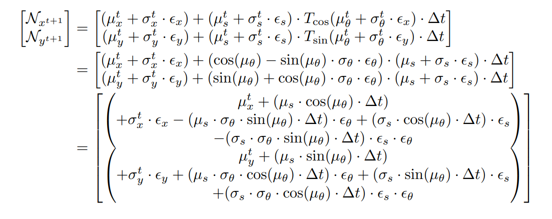
A. Full Expansion of Formulation 3
\ 
\
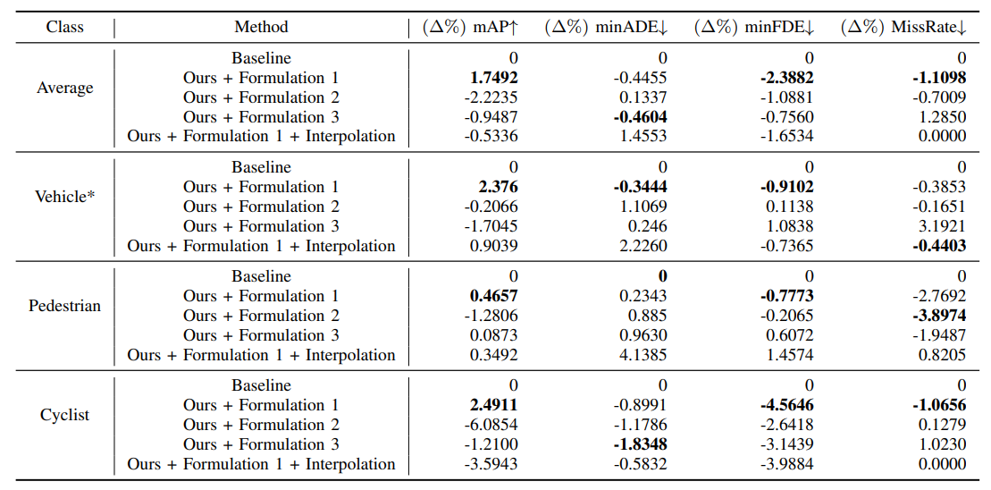
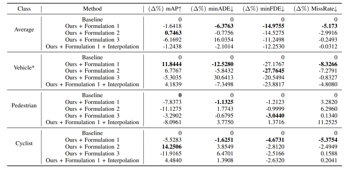
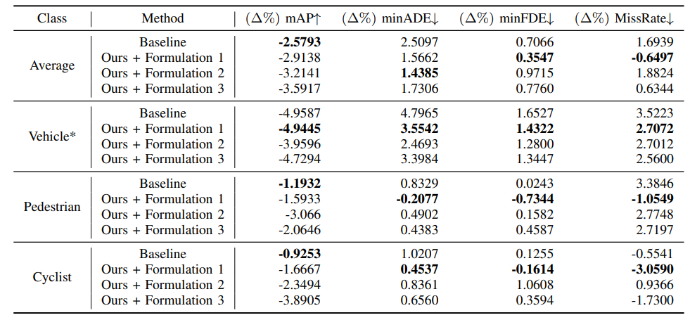
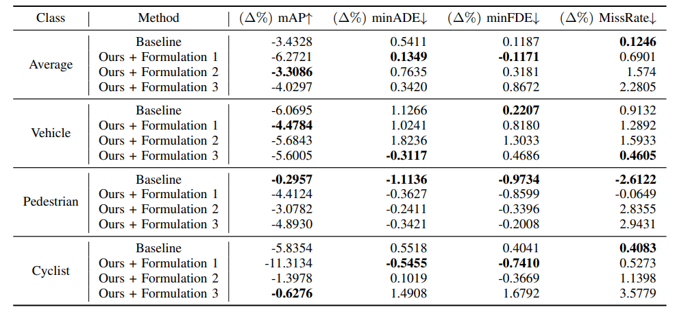
B. Additional Results By Class
In the paper, we present results on vehicles since we use kinematic models based on vehicles as priors. Here, we present the full results per-class for each experiment in Tables IV, V, VI, and VII. The results reported in the paper are starred (*), which are re-iterated below for full context.
\ 
\ 
\ 
\ 
\ \
C. Experiment Hyperparameters
\ 
\
:::info Authors:
(1) Laura Zheng, Department of Computer Science, University of Maryland at College Park, MD, U.S.A (lyzheng@umd.edu);
(2) Sanghyun Son, Department of Computer Science, University of Maryland at College Park, MD, U.S.A (shh1295@umd.edu);
(3) Jing Liang, Department of Computer Science, University of Maryland at College Park, MD, U.S.A (jingl@umd.edu);
(4) Xijun Wang, Department of Computer Science, University of Maryland at College Park, MD, U.S.A (xijun@umd.edu);
(5) Brian Clipp, Kitware (brian.clipp@kitware.com);
(6) Ming C. Lin, Department of Computer Science, University of Maryland at College Park, MD, U.S.A (lin@umd.edu).
:::
:::info This paper is available on arxiv under ATTRIBUTION-NONCOMMERCIAL-NODERIVS 4.0 INTERNATIONAL license.
:::
\
You May Also Like

Taiko and Chainlink to Unleash Reliable Onchain Data for DeFi Ecosystem

Why The Green Bay Packers Must Take The Cleveland Browns Seriously — As Hard As That Might Be
